Advanced Usage
These tutorials give some examples in the use of the
underlying radvel API.
They are also available as interactive iPython notebooks
in the tests subdirectory of the radvel package.
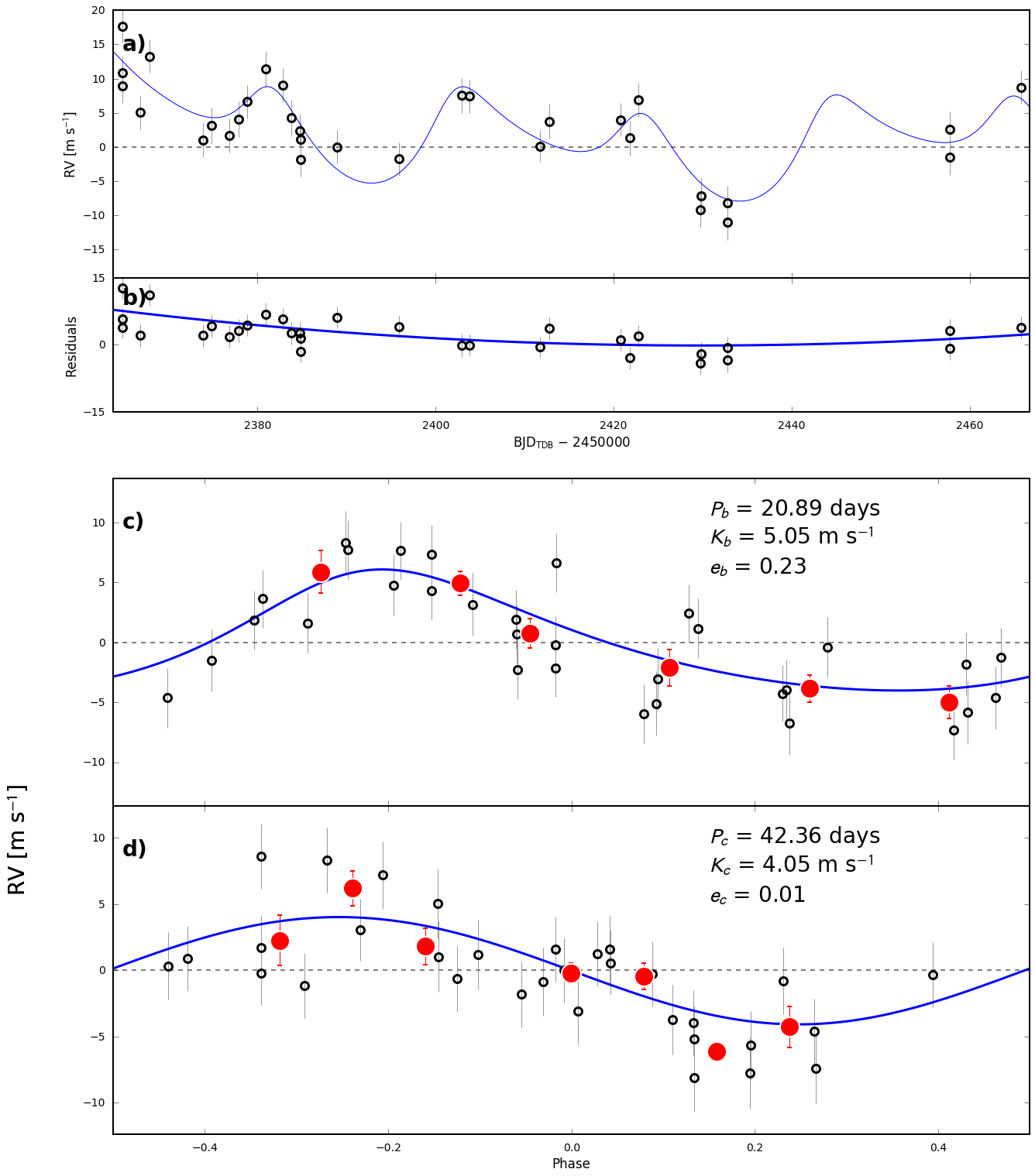
K2-24 Fitting & MCMC
Using the K2-24 (EPIC-203771098) dataset, we demonstrate how to use the
radvel API to:
- perform a max-likelihood fit
- do an MCMC exploration of the posterior space
- plot the results
Perform some preliminary imports:
import os

import matplotlib
import numpy as np
import pylab as pl
import pandas as pd
from scipy import optimize

import corner

import radvel
import radvel.plotting
Define a function that we will use to initialize the
radvel.Parameters and radvel.RVModel objects
def initialize_model():
    time_base = 2420
    params = radvel.Parameters(2,basis='per tc secosw sesinw logk') # number of planets = 2
    params['per1'] = radvel.Parameter(value=20.885258)
    params['tc1'] = radvel.Parameter(value=2072.79438)
    params['secosw1'] = radvel.Parameter(value=0.01)
    params['sesinw1'] = radvel.Parameter(value=0.01)
    params['logk1'] = radvel.Parameter(value=1.1)
    params['per2'] = radvel.Parameter(value=42.363011)
    params['tc2'] = radvel.Parameter(value=2082.62516)
    params['secosw2'] = radvel.Parameter(value=0.01)
    params['sesinw2'] = radvel.Parameter(value=0.01)
    params['logk2'] = radvel.Parameter(value=1.1)
    mod = radvel.RVModel(params, time_base=time_base)
    mod.params['dvdt'] = radvel.Parameter(value=-0.02)
    mod.params['curv'] = radvel.Parameter(value=0.01)
    return mod
Define a simple plotting function to display the data and model.
def plot_results(like):
    fig = pl.figure(figsize=(12,4))
    fig = pl.gcf()
    fig.set_tight_layout(True)
    pl.errorbar(
        like.x, like.model(t)+like.residuals(),
        yerr=like.yerr, fmt='o'
        )
    pl.plot(ti, like.model(ti))
    pl.xlabel('Time')
    pl.ylabel('RV')
    pl.draw()
Load up the K2-24 data. In this example the RV data is stored in an CSV file
path = os.path.join(radvel.DATADIR,'epic203771098.csv')
rv = pd.read_csv(path)

t = np.array(rv.t)
vel = np.array(rv.vel)
errvel = rv.errvel
ti = np.linspace(rv.t.iloc[0]-5,rv.t.iloc[-1]+5,100)
Circular Orbits
Use the function we just defined to initialize a model object and add a few additional parameters
into the radvel.likelihood.Likelihood object that are not associated with the Keplerian orbital model
but still needed to calculate a likelihood.
mod = initialize_model()
like = radvel.likelihood.RVLikelihood(mod, t, vel, errvel)
like.params['gamma'] = radvel.Parameter(value=0.1)
like.params['jit'] = radvel.Parameter(value=1.0)
Choose which parameters to vary or fix. By default, all radvel.Parameter objects will vary,
so you only have to worry about setting the ones you want to hold fixed.
like.params['secosw1'].vary = False
like.params['sesinw1'].vary = False
like.params['secosw2'].vary = False
like.params['sesinw2'].vary = False
like.params['per1'].vary = False
like.params['per2'].vary = False
like.params['tc1'].vary = False
like.params['tc2'].vary = False
print(like)
parameter                     value      vary
per1                        20.8853      False
tc1                         2072.79      False
secosw1                        0.01      False
sesinw1                        0.01      False
logk1                           1.1       True
per2                         42.363      False
tc2                         2082.63      False
secosw2                        0.01      False
sesinw2                        0.01      False
logk2                           1.1       True
dvdt                          -0.02       True
curv                           0.01       True
gamma                           0.1       True
jit                               1       True
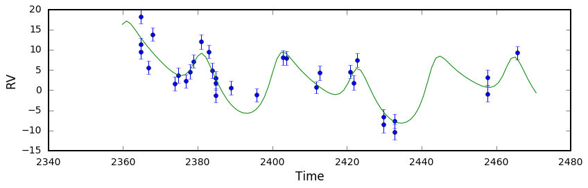
Plot the initial model
pl.figure()
plot_results(like)
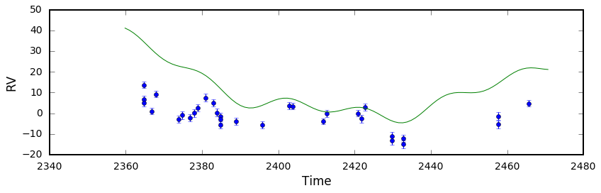
Well that solution doesn’t look very good. Now lets try to optimize the parameters set to vary by maximizing the likelihood.
Initialize a radvel.Posterior object and add some priors
post = radvel.posterior.Posterior(like)
post.priors += [radvel.prior.Gaussian( 'jit', np.log(3), 0.5)]
post.priors += [radvel.prior.Gaussian( 'logk2', np.log(5), 10)]
post.priors += [radvel.prior.Gaussian( 'logk1', np.log(5), 10)]
post.priors += [radvel.prior.Gaussian( 'gamma', 0, 10)]
Maximize the likelihood and print the updated posterior object
res  = optimize.minimize(
    post.neglogprob_array,     # objective function is negative log likelihood
    post.get_vary_params(),    # initial variable parameters
    method='Powell',           # Nelder-Mead also works
    )

plot_results(like)             # plot best fit model
print(post)
parameter                     value      vary
per1                        20.8853      False
tc1                         2072.79      False
secosw1                        0.01      False
sesinw1                        0.01      False
logk1                       1.56037       True
per2                         42.363      False
tc2                         2082.63      False
secosw2                        0.01      False
sesinw2                        0.01      False
logk2                       1.80937       True
dvdt                     -0.0364432       True
curv                    -0.00182455       True
jit                         2.62376       True
gamma                       2.62376       True

Priors
------
Gaussian prior on jit, mu=1.09861228867, sigma=0.5
Gaussian prior on logk2, mu=1.60943791243, sigma=10
Gaussian prior on logk1, mu=1.60943791243, sigma=10
Gaussian prior on gamma, mu=0, sigma=10
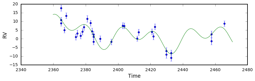
That looks much better!
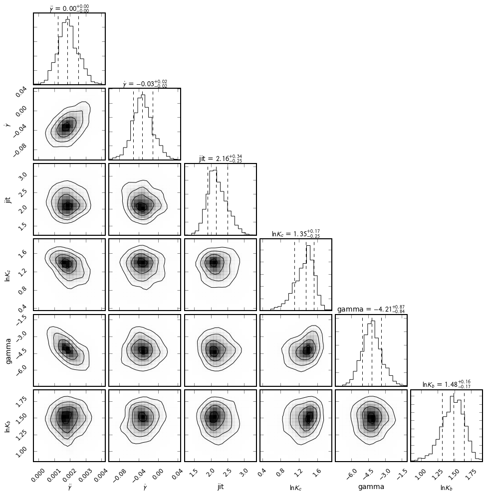
Now lets use Markov-Chain Monte Carlo (MCMC) to estimate the parameter uncertainties. In this example we will run 1000 steps for the sake of speed but in practice you should let it run at least 10000 steps and ~50 walkers. If the chains converge before they reach the maximum number of allowed steps it will automatically stop.
df = radvel.mcmc(post,nwalkers=20,nrun=1000)
Make a corner plot to display the posterior distributions.
radvel.plotting.corner_plot(post, df)
Eccentric Orbits
Allow secosw and sesinw parameters to vary
like.params['secosw1'].vary = True
like.params['sesinw1'].vary = True
like.params['secosw2'].vary = True
like.params['sesinw2'].vary = True
Add an EccentricityPrior to ensure that eccentricity stays below
1.0. In this example we will also add a Gaussian prior on the jitter
(jit) parameter with a center at 2.0 m/s and a width of 0.1 m/s.
post = radvel.posterior.Posterior(like)
post.priors += [radvel.prior.EccentricityPrior( 2 )]
post.priors += [radvel.prior.Gaussian( 'jit', np.log(2), np.log(0.1))]
Optimize the parameters by maximizing the likelihood and plot the result
res  = optimize.minimize(
    post.neglogprob_array,
    post.get_vary_params(),
    method='Nelder-Mead',)

plot_results(like)
print(post)
parameter                     value      vary
per1                        20.8853      False
tc1                         2072.79      False
secosw1                    0.389104       True
sesinw1                    0.059227       True
logk1                       1.65139       True
per2                         42.363      False
tc2                         2082.63      False
secosw2                    0.194769       True
sesinw2                   -0.422685       True
logk2                        1.6278       True
dvdt                      -0.027433       True
curv                     0.00152703       True
gamma                      -4.38996       True
jit                          2.2025       True

Priors
------
e1 constrained to be < 0.99
e2 constrained to be < 0.99
Gaussian prior on jit, mu=0.6931471805599453, sigma=-2.3025850929940455
Plot the final solution
radvel.plotting.rv_multipanel_plot(post)