Getting Started
Installation
While it is possible to install radvel inside a minimal Python environment like that built-in to Mac OSX,
we recommend first installing a scientific Python environment such as
Anaconda or Miniconda.
Install radvel using pip:
$ pip install radvel
Note: If you encounter compilation issues on macOS (especially with newer Xcode versions), consider using conda for problematic dependencies:
$ conda install pytables h5py
$ pip install radvel
Make sure that pdflatex is installed and in your system’s path.
You can get pdflatex by installing the TexLive package or other LaTeX distributions.
By default it is expected to be in your system’s path, but you may
specify a path to pdflatex using the --latex-compiler
option at the radvel report step.
Build System
radvel uses a modern build system based on pyproject.toml and hatchling instead of the deprecated setuptools.
This provides faster builds and better dependency management. The build system automatically handles:
Cython extensions compilation
Python version compatibility (3.8+)
Modern dependency resolution
Automatic version detection from source code
If you are running OSX, and want to perform Gaussian Process likelihood computations in parallel, you may need to perform some additional installation steps. See multiprocessing on OSX.
Development Installation
To install radvel in development mode for contributing to the codebase:
$ git clone https://github.com/California-Planet-Search/radvel.git
$ cd radvel

# Install problematic dependencies via conda (recommended for macOS)
$ conda install pytables h5py

# Install radvel in development mode
$ pip install -e .
If you wish to use the celerite GP kernels you will also need to install celerite. See the celerite install instructions.
Continuous Integration
radvel uses GitHub Actions for continuous integration, testing on multiple Python versions (3.8, 3.9, 3.11, 3.12).
The CI system automatically:
Runs tests on all supported Python versions
Builds and validates the package
Generates coverage reports
Publishes to PyPI on releases
For local testing, you can run the test suite with:
$ nosetests radvel --with-coverage --cover-package=radvel
To use nested sampling packages other than the default UltraNest sampler, you will also need to install them. Other samplers implemented in Radvel are:
See Available Nested Samplers for more details.
Example Fit
Test your installation by running through one of the included
examples. We will use the radvel command line interface to execute
a multi-planet, multi-instrument fit.
The radvel binary should have been automatically placed in your system’s path by the
pip command (see Installation). If your system can not find
the radvel executable then try running python setup.py install
from within the top-level radvel directory.
First lets look at radvel --help for the available options:
$ radvel --help
usage: RadVel [-h] [--version] {fit,plot,mcmc,ns,derive,bic,table,report} ...

RadVel: The Radial Velocity Toolkit

optional arguments:
  -h, --help            show this help message and exit
  --version             Print version number and exit.

subcommands:
  {fit,plot,mcmc,ns,derive,bic,table,report}
Here is an example workflow to
run a simple fit using the included HD164922.py example
configuration file. This example configuration file can be found in the example_planets
subdirectory on the GitHub repository page.
Perform a maximum-likelihood fit. You almost always will need to do this first:
$ radvel fit -s /path/to/radvel/example_planets/HD164922.py
By default the results will be placed in a directory with the same name as
your planet configuration file (without .py, e.g. HD164922). You
may also specify an output directory using the -o flag.
After the maximum-likelihood fit is complete the directory should have been created
and should contain one new file:
HD164922/HD164922_post_obj.pkl. This is a pickle binary file
that is not meant to be human-readable but lets make a plot of the
best-fit solution contained in that file:
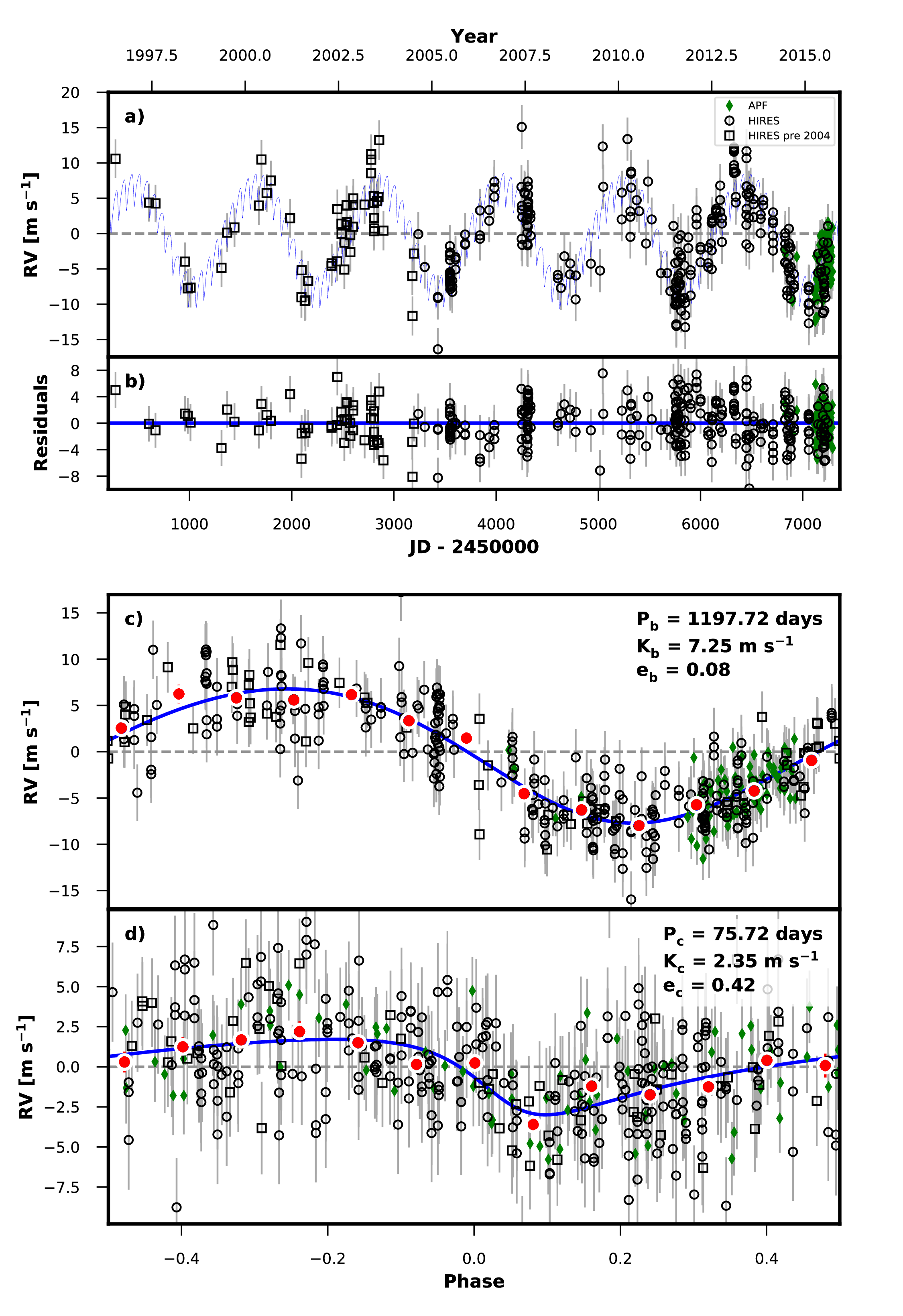
$ radvel plot -t rv -s /path/to/radvel/example_planets/HD164922.py
This should produce a plot named HD164922_rv_multipanel.pdf that looks something like this.
Next lets perform the Markov-Chain Monte Carlo (MCMC) exploration to assess parameter uncertainties.
Next, we can sample the posterior distribution to assess parameter uncertainties. RadVel can do this either with Markov Chain Monte Carlo (MCMC) or nested sampling (NS).
MCMC is available with the mcmc subcommand.
$ radvel mcmc -s /path/to/radvel/example_planets/HD164922.py
Once the MCMC chains finish running there will be another new file called HD164922_mcmc_chains.csv.tar.bz2. This is a compressed csv file containing the parameter values and likelihood at each step in the MCMC chains.
Nested sampling is available through the ns subcommand.
$ radvel ns -s /path/to/radvel/example_planets/HD164922.py
See radvel ns --help for a full list of available options.
After nested sampling has run, the equal weight (equivalent to MCMC)
chains from nested sampling are stored in HD164922_chains_ns.csv.bz2.
All subsequent steps steps can be run with either MCMC or nested sampling chains.
By default, MCMC will be used if available and otherwise nested sampling will be used.
The --sampler argument allows us to specify which chains to use.
Note that the trend and auto plots are only available for MCMC.
One of the main advantages of nested sampling is that it provides the Bayesian evidence.
The RadVel CLI does not implement model comparison with the evidence, but the
nested sampling results are saved under HD164922_ns/results.hdf5 and can
be accessed with radvel.nested_sampling.load_results(). See the TOI-141 tutorial for an example that includes model comparison.
Once the sampling is finished, we can update the RV time series plot and generate the full suite of plots.
$ radvel plot -t rv corner trend -s /path/to/radvel/example_planets/HD164922.py
We can summarize our analysis with the radvel report command.
$ radvel report -s /path/to/radvel/example_planets/HD164922.py
which creates a LaTeX document and corresponding PDF to summarize the results. Note that this command assembles values and plots that have been computed through other commands, if you want to update, rerun the previous commands before reruning radvel report
The report PDF will be saved as HD164922_results.pdf. It should contain a table reporting the parameter values and uncertainties, a table summarizing the priors, the RV time-series plot, and a corner plot showing the posterior distributions for all free parameters.
Optional Features
Combine the measured properties of the RV time-series with the properties of the host star defined in the setup file to derive physical parameters for the planetary system. Have a look at the epic203771098.py example setup file to see how to include stellar parameters.
$ radvel derive -s /path/to/radvel/example_planets/HD164922.py
Generate a corner plot for the derived parameters. This plot will also be included in the summary report if available.
$ radvel plot -t derived -s /path/to/radvel/example_planets/HD164922.py
Perform a model comparison testing models eliminating different sets of planets, their eccentricities, and RV trends. If this is run a new table will be included in the summary report.
$ radvel ic -t nplanets e trend -s /path/to/radvel/example_planets/HD164922.py
Generate and save only the TeX code for any/all of the tables.
$ radvel table -t params priors ic_compare derived -s /path/to/radvel/example_planets/HD164922.py