K2-24 Fitting & MCMC
Using the K2-24 (EPIC-203771098) dataset, we demonstrate how to use the radvel API to:
perform a max-likelihood fit
do an MCMC exploration of the posterior space
plot the results
Circular Orbits
Perform some preliminary imports:
[1]:
%matplotlib inline

import os

import matplotlib
import numpy as np
import pylab as pl
import pandas as pd
from scipy import optimize

import corner

import radvel
import radvel.likelihood
from radvel.plot import orbit_plots, mcmc_plots

matplotlib.rcParams['font.size'] = 14
Define a function that we will use to initialize the radvel.Parameters and radvel.RVModel objects
[2]:
def initialize_model():
    time_base = 2420
    params = radvel.Parameters(2,basis='per tc secosw sesinw logk') # number of planets = 2
    params['per1'] = radvel.Parameter(value=20.885258)
    params['tc1'] = radvel.Parameter(value=2072.79438)
    params['secosw1'] = radvel.Parameter(value=0.01)
    params['sesinw1'] = radvel.Parameter(value=0.01)
    params['logk1'] = radvel.Parameter(value=1.1)
    params['per2'] = radvel.Parameter(value=42.363011)
    params['tc2'] = radvel.Parameter(value=2082.62516)
    params['secosw2'] = radvel.Parameter(value=0.01)
    params['sesinw2'] = radvel.Parameter(value=0.01)
    params['logk2'] = radvel.Parameter(value=1.1)
    mod = radvel.RVModel(params, time_base=time_base)
    mod.params['dvdt'] = radvel.Parameter(value=-0.02)
    mod.params['curv'] = radvel.Parameter(value=0.01)
    return mod
Define a simple plotting function to display the data, model, and residuals
[3]:
def plot_results(like):
    fig = pl.figure(figsize=(12,4))
    fig = pl.gcf()
    pl.errorbar(
        like.x, like.model(t)+like.residuals(),
        yerr=like.yerr, fmt='o'
        )
    pl.plot(ti, like.model(ti))
    pl.xlabel('Time')
    pl.ylabel('RV')
    pl.draw()
    fig.tight_layout()
Load up the K2-24 data. In this example the RV data and parameter starting guesses are stored in an csv file
[4]:
path = os.path.join(radvel.DATADIR,'epic203771098.csv')
rv = pd.read_csv(path)

t = np.array(rv.t)
vel = np.array(rv.vel)
errvel = rv.errvel
ti = np.linspace(rv.t.iloc[0]-5,rv.t.iloc[-1]+5,100)
Fit the K2-24 RV data assuming:
circular orbits
fixed period, time of transit
Set initial guesses for the parameters. Setting vary=False and linear=True on the gamma parameters will cause them to be solved for analytically following the technique described here (Thanks Tim Brandt!). If you use this you will need to calculate the uncertainties on gammas manually following that derivation.
[5]:
mod = initialize_model()
like = radvel.likelihood.RVLikelihood(mod, t, vel, errvel)
like.params['gamma'] = radvel.Parameter(value=0.1, vary=False, linear=True)
like.params['jit'] = radvel.Parameter(value=1.0)
Choose which parameters to vary or fix. By default, all radvel.Parameter objects will vary, so you only have to worry about setting the ones you want to hold fixed.
[6]:
like.params['secosw1'].vary = False
like.params['sesinw1'].vary = False
like.params['secosw2'].vary = False
like.params['sesinw2'].vary = False
like.params['per1'].vary = False
like.params['per2'].vary = False
like.params['tc1'].vary = False
like.params['tc2'].vary = False
print(like)
parameter                     value      vary
per1                        20.8853      False
tc1                         2072.79      False
secosw1                        0.01      False
sesinw1                        0.01      False
logk1                           1.1       True
per2                         42.363      False
tc2                         2082.63      False
secosw2                        0.01      False
sesinw2                        0.01      False
logk2                           1.1       True
dvdt                          -0.02       True
curv                           0.01       True
gamma                           0.1      False
jit                               1       True
tp1                         2070.18
e1                           0.0002
w1                         0.785398
k1                          3.00417
tp2                         2077.33
e2                           0.0002
w2                         0.785398
k2                          3.00417
Plot the initial model
[7]:
pl.figure()
plot_results(like)
<Figure size 640x480 with 0 Axes>
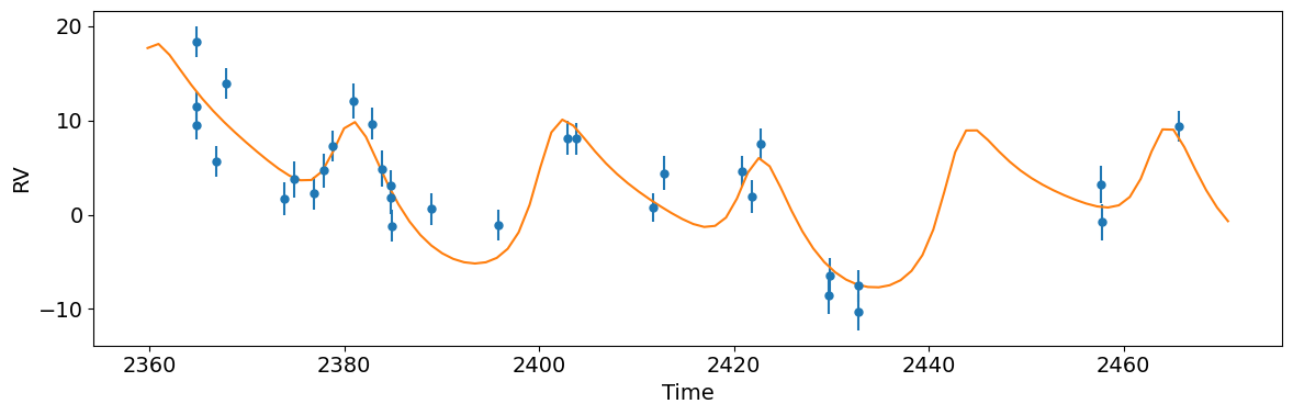
Well that solution doesn’t look very good. Now lets try to optimize the parameters set to vary by maximizing the likelihood.
Initialize a radvel.Posterior object and add some priors
[8]:
post = radvel.posterior.Posterior(like)
post.priors += [radvel.prior.Gaussian( 'jit', np.log(3), 0.5)]
post.priors += [radvel.prior.Gaussian( 'logk2', np.log(5), 10)]
post.priors += [radvel.prior.Gaussian( 'logk1', np.log(5), 10)]
post.priors += [radvel.prior.Gaussian( 'gamma', 0, 10)]
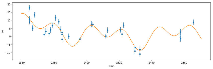
Maximize the likelihood and print the updated posterior object
[9]:
res  = optimize.minimize(
    post.neglogprob_array,     # objective function is negative log likelihood
    post.get_vary_params(),    # initial variable parameters
    method='Nelder-Mead',           # Powell also works
    )

plot_results(like)             # plot best fit model
print(post)
parameter                     value      vary
per1                        20.8853      False
tc1                         2072.79      False
secosw1                        0.01      False
sesinw1                        0.01      False
logk1                        1.5503       True
per2                         42.363      False
tc2                         2082.63      False
secosw2                        0.01      False
sesinw2                        0.01      False
logk2                       1.36832       True
dvdt                     -0.0295124       True
curv                     0.00183616       True
gamma                        -4.013      False
jit                         2.08458       True
tp1                         2070.18
e1                           0.0002
w1                         0.785398
k1                          4.71289
tp2                         2077.33
e2                           0.0002
w2                         0.785398
k2                          3.92875

Priors
------
Gaussian prior on jit, mu=1.0986122886681096, sigma=0.5
Gaussian prior on logk2, mu=1.6094379124341003, sigma=10
Gaussian prior on logk1, mu=1.6094379124341003, sigma=10
Gaussian prior on gamma, mu=0, sigma=10
That looks much better!
Now lets use Markov-Chain Monte Carlo (MCMC) to estimate the parameter uncertainties. In this example we will run 400 steps for the sake of speed but in practice you should let it run at least 10000 steps and ~50 walkers. If the chains converge before they reach the maximum number of allowed steps it will automatically stop.
[10]:
df = radvel.mcmc(post,nwalkers=50,nrun=10000,savename='rawchains.h5')
200000/4000000 (5.0%) steps complete; Running 21445.43 steps/s; Mean acceptance rate = 55.4%; Min Auto Factor =  75; Max Auto Relative-Change =   inf; Min Tz = 18327.9; Max G-R = 1.002
Discarding burn-in now that the chains are marginally well-mixed

460000/4000000 (11.5%) steps complete; Running 17740.35 steps/s; Mean acceptance rate = 55.0%; Min Auto Factor =  90; Max Auto Relative-Change = 0.0245; Min Tz = 16833.8; Max G-R = 1.002
Chains are well-mixed after 460000 steps! MCMC completed in 23.4 seconds
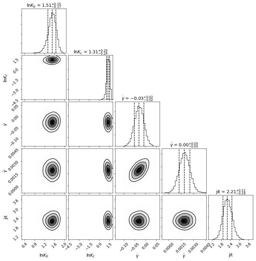
Now lets make a corner plot to display the posterior distributions.
[11]:
Corner = mcmc_plots.CornerPlot(post, df)
Corner.plot()
Eccentric Orbits
Allow secosw and sesinw parameters to vary
[12]:
like.params['secosw1'].vary = True
like.params['sesinw1'].vary = True
like.params['secosw2'].vary = True
like.params['sesinw2'].vary = True
Add an EccentricityPrior to ensure that eccentricity stays below 1.0. In this example we will also add a Gaussian prior on the jitter (jit) parameter with a center at 2.0 m/s and a width of 0.1 m/s.
[13]:
post = radvel.posterior.Posterior(like)
post.priors += [radvel.prior.EccentricityPrior( 2 )]
post.priors += [radvel.prior.Gaussian( 'jit', np.log(2), np.log(0.1))]
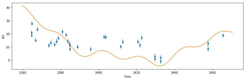
Optimize the parameters by maximizing the likelihood and plot the result.
The warning about an invalid value can be safely ignored.
[14]:
res  = optimize.minimize(
    post.neglogprob_array,
    post.get_vary_params(),
    method='Powell'
)

plot_results(like)
print(post)
parameter                     value      vary
per1                        20.8853      False
tc1                         2072.79      False
secosw1                    0.398562       True
sesinw1                   -0.403908       True
logk1                       1.81293       True
per2                         42.363      False
tc2                         2082.63      False
secosw2                     -0.1305       True
sesinw2                    0.367332       True
logk2                       1.48343       True
dvdt                     -0.0299603       True
curv                     0.00205612       True
gamma                      -4.51743      False
jit                           1.956       True
tp1                         2066.73
e1                         0.321993
w1                        -0.792059
k1                          6.12836
tp2                         2084.31
e2                         0.151963
w2                          1.91215
k2                          4.40803

Priors
------
e1 constrained to be < 0.99
e2 constrained to be < 0.99
Gaussian prior on jit, mu=0.6931471805599453, sigma=-2.3025850929940455
invalid value encountered in scalar multiply
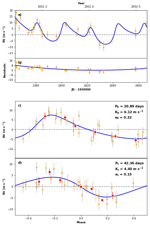
Plot the final solution
[15]:
RVPlot = orbit_plots.MultipanelPlot(post, legend=False)
RVPlot.plot_multipanel()
[15]:
(<Figure size 750x1092.86 with 5 Axes>,
 [<Axes: ylabel='RV [m s$^{\\mathregular{-1}}$]'>,
  <Axes: xlabel='JD - 2450000', ylabel='Residuals'>,
  <Axes: xlabel='Phase', ylabel='RV [m s$^{\\mathregular{-1}}$]'>,
  <Axes: xlabel='Phase', ylabel='RV [m s$^{\\mathregular{-1}}$]'>])